Real-data example

This example runs a GreyRing inference on public gravitational-wave strain data using Bilby.

The goal is to show how the GreyRing waveform can be plugged into a standard Bilby likelihood.

Folder

examples/real_data/

Typical structure:

examples/real_data/
  run.py
  theory/
    Zed_abs.txt
    Zed_phase.txt

The greybody tables must be placed in:

examples/real_data/theory/

with names:

Zed_abs.txt
Zed_phase.txt

See Theory files for the table format.

Waveform generator

To use the GreyRing waveform generator, the package must be imported in the analysis script.

For example:

from greyring.model import greyring_22_free_ampl_phase

The example uses a dedicated GreyRing frequency-domain waveform model for real data. In Bilby, the waveform generator is built schematically as:

waveform_generator = bilby.gw.WaveformGenerator(
    frequency_domain_source_model=greyring_22_free_ampl_phase,
    parameter_conversion=identity_map_conversion,
    waveform_arguments={},
)

The source model returns the detector-frame frequency-domain polarizations:

h_plus(f), h_cross(f)

for the selected GreyRing parameters. Additional informations can be found in the README file in the examples folder.

GreyRing parameters

Besides the standard event-level quantities, the GreyRing model samples the remnant intrinsic parameters and the phenomenological ringdown coefficients.

In the example, phase and time are marginalized over in the likelihood.

Priors

A minimal real-data run usually needs priors on Mf, af, A, p, and c, in addition to the standard Bilby priors required by the likelihood setup.

A typical choice for the model parameters is:

priors["A"] = bilby.core.prior.LogUniform(minimum=0.01, maximum=15, name="A")
priors["p"] = bilby.core.prior.Uniform(minimum=-0.5, maximum=1.5, name="p")
priors["c"] = bilby.core.prior.Uniform(minimum=0.0, maximum=3.0, name="c")

The numerical ranges should be adapted to the event, the frequency band, and the normalization convention used in the waveform model. See details in the paper.

Run

From the repository root:

cd examples/real_data
python run.py

The script downloads the strain data, estimates the PSD, builds the interferometers and likelihood, and runs Dynesty through Bilby.

Example result

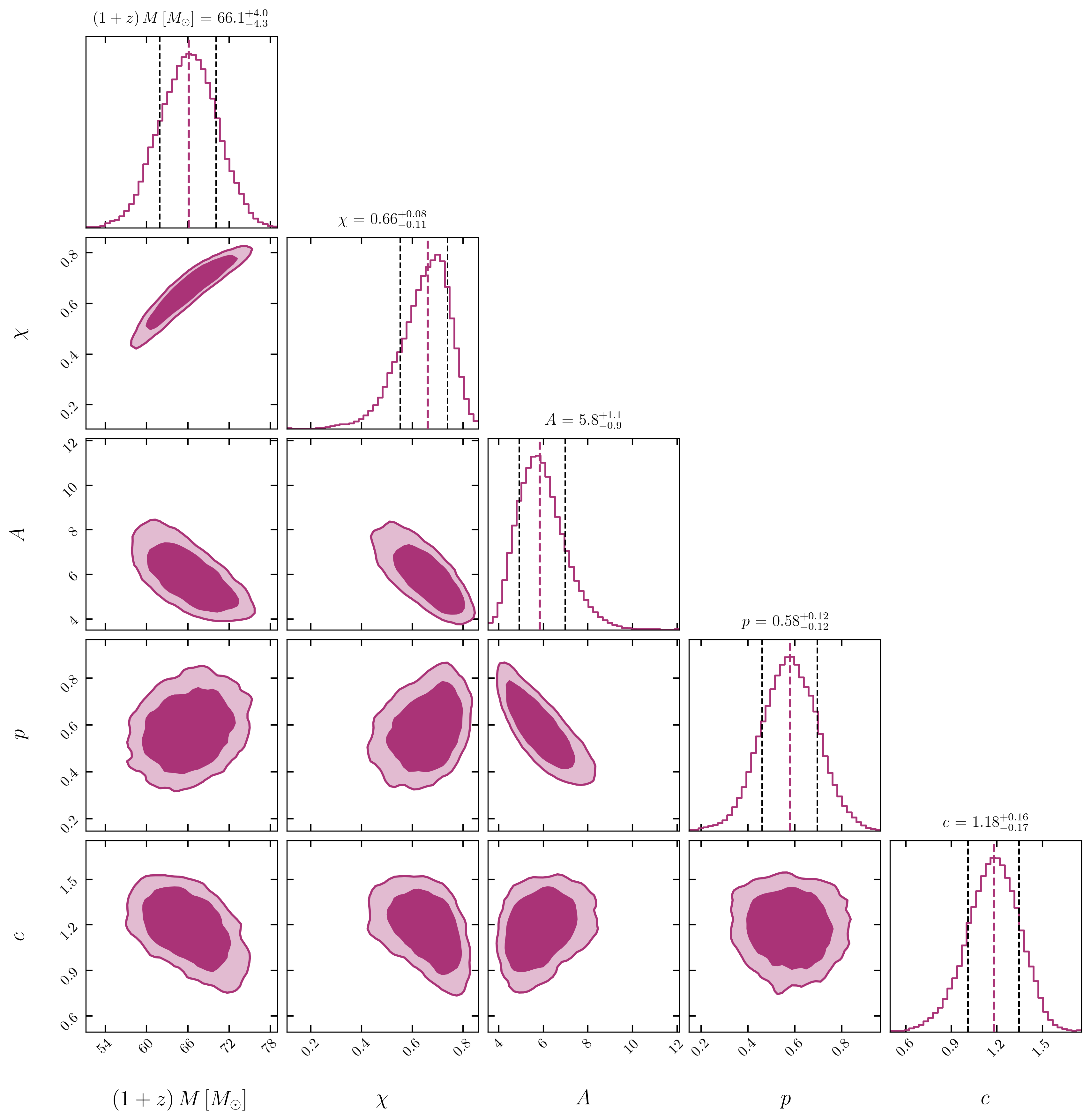
The plot shows a representative GreyRing posterior obtained from the analysis of GW250114 in the paper.