SXS fit example

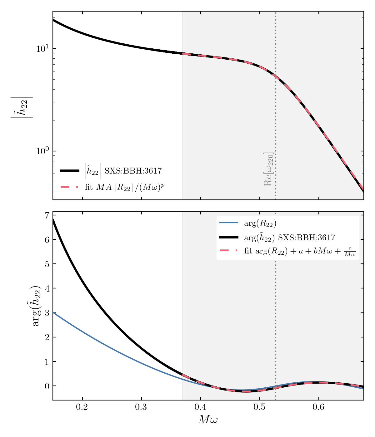
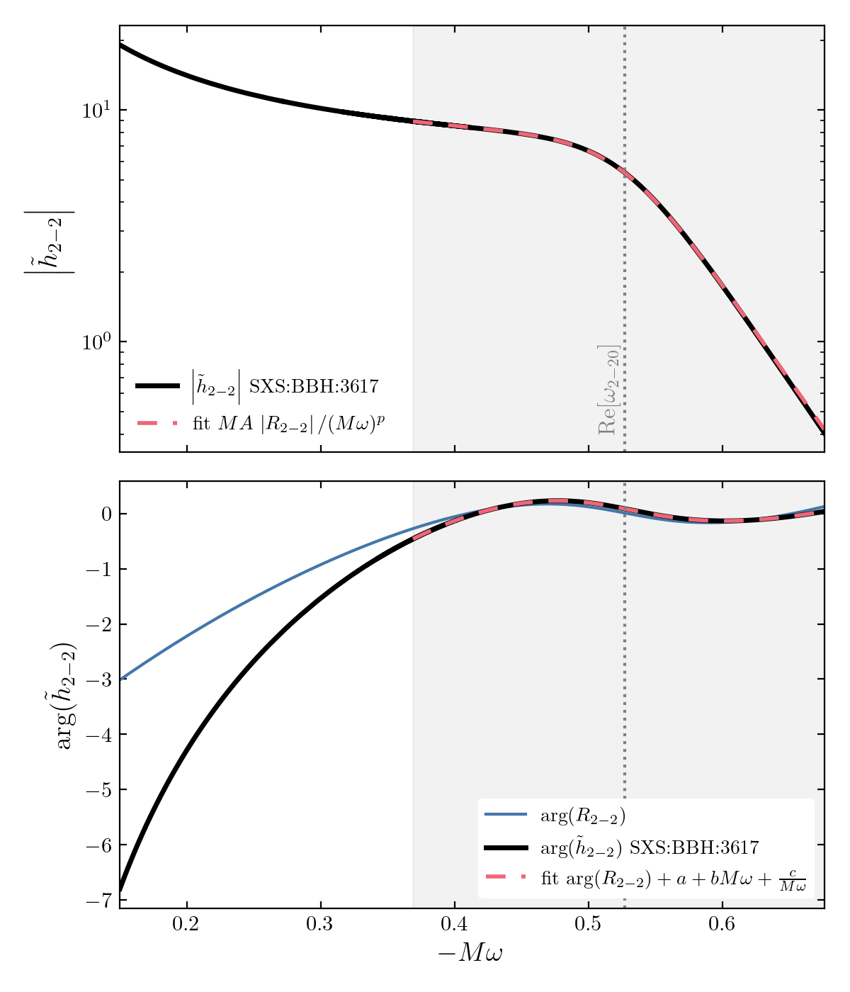
This example fits the GreyRing model directly to a numerical-relativity waveform from the SXS catalog.

The user selects an SXS simulation and a multipole (ℓ, m). The code extracts the corresponding waveform mode, builds the frequency-domain spectrum, fits the GreyRing amplitude and phase, and computes the mismatch.

Folder

examples/sxs_fit/

Typical structure:

examples/sxs_fit/
  run.py
  theory/
    dataAbs22.txt
    dataPhase22.txt

Theory files

The example requires two theory files:

dataAbs22.txt
dataPhase22.txt

They contain the absolute value and phase of the complex reflectivity for the (l, m)=(2,2) mode.

Each file should contain a Python-style array named:

ZedSIM = [...]

with comma-separated entries. Here SIM is the SXS simulation ID. For example, for SXS:BBH:3617, the expected array name is:

Zed3617 = [...]

The length of this array must match the omega_theory array passed to gr.fit.

At the moment, the example can be tested for multipoles up to ℓ = 4. For negative-m modes, compute the reflectivity for the corresponding positive-m mode. The code expects the theory file label to use the positive-m convention. For example, a fit of the (2, -2) mode uses theory files labelled as (2, 2).

See Theory files for more details.

Minimal usage

import numpy as np
import greyring as gr

omega_theory = np.linspace(0.001, 1.2, 1200)

result = gr.fit(
    sim_number=3617,
    ell=2,
    m=2,
    abs_file="theory/dataAbs22.txt",
    phase_file="theory/dataPhase22.txt",
    omega_theory=omega_theory,
    omega_i_factor=0.7,
    omega_f_amp_ratio=20.0,
    make_plot=True,
)

print(result.A)
print(result.p)
print(result.c)
print(result.mismatch)

Main inputs

Parameter	Meaning
`sim_number`	SXS simulation number
`ell`, `m`	waveform multipole
`abs_file`	reflectivity absolute-value file
`phase_file`	reflectivity phase file
`omega_theory`	frequency array corresponding to the reflectivity arrays
`omega_i_factor`	lower edge of the fitting window, relative to the knee frequency
`omega_f_amp_ratio`	upper edge of the fitting window, set by the amplitude-drop criterion
`make_plot`	save a diagnostic plot

Fit window

The lower edge is defined as

omega_i = omega_i_factor * omega_x

where omega_x is the knee frequency.

The upper edge is selected from

|h(omega_f)| = |h(omega_x)| / omega_f_amp_ratio

The default choice is

omega_i_factor = 0.7
omega_f_amp_ratio = 20.0

See details in the paper.

Example figures

Example diagnostic plots for the (2, 2) and (2, -2) modes are included in the example folder.

SXS fit diagnostic plot for the (2, 2) mode